It's been quite a long time since my last post and returning to this media, I'll try to publish technical stuff now more related to Deep Learning. In this one, I'd like to share a collection of Jupyter Notebooks I've created for a tutorial on the basics of Neural Networks and Deep Learning, aimed at teaching the main concepts through code.
I used Jupyter Notebooks, knowing that this is a
great tool for communicating ideas, diagrams, and code in the same
place. But I also wanted to make the process easier for the attendants,
so I hosted those notebooks in Azure Notebooks, which is a fantastic
platform for Notebooks-As-A-Service. In this way, attendants didn't need
to install anything. Just logging into the service (for free) through a
web browser and cloning my library allowed them to run all experiments.
For anyone that wants to play with that: just go to the Azure Notebooks
web page and sign in with your Microsoft account (or create a new one
for free following the instructions in the sign in window, in case you
don't have one yet). Then just clone my library to your account and
start running the tutorials. It can be cloned from here: https://notebooks.azure.com/vilcek/libraries/deeplearning-very-basics

This blog is about data, in a computational sense. Small and Big. Simple and Complex. And how to deal with it.
Tuesday, April 24, 2018
Friday, February 6, 2015
Machine Learning with H2O on Hadoop
Introduction
Machine learning on Hadoop has evolved a lot since the debut of Apache Mahout. Back then, a data scientist had to be able to understand at least some basics of Java programming and Linux shell scripting in order to assemble more complex MapReduce jobs and take the most of Mahout. And Mahout is batch-only oriented, which makes it difficult for interactive, data exploratory analysis. But now, machine learning at scale on top of Hadoop is getting a lot of traction with new-generation machine learning frameworks. By embracing YARN, those are not tied only to the MapReduce paradigm anymore and are capable of in-memory data processing. Some examples from this new generation are Apache Spark’s MLlib and Oxdata’s H2O. Moreover, Mahout is being ported to take advantage of those new frameworks as is shown in the “Mahout News” section of its home page.
In this tutorial I will show how to install H2O on a Hadoop
cluster and run some basic machine learning tasks. For the Hadoop cluster
environment I will use Hortonworks 2.1 Sandbox VM. And for H2O, I will use the
H2o driver specific for HDP 2.1 from the latest stable release.
1. Download and Install HDP Sandbox VM
Download and install the Hortonworks Sandbox VM. Note: as of this writing, it seems that H2O is not properly running on the latest HDP Sandbox VM, which is version 2.2. For this tutorial I used HDP Sandbox version 2.1, which can be downloaded from here.
2. Download and Install H2O on the HDP Sandbox VM
Log in your HDP Sandbox VM:
ssh
root@<your-hdp-sandbox-ip-address> -p 22
Create a directory for H2O download and installation:
# cd /opt
# mkdir h2o
# cd
h2o
Check for H2O latest stable release here and click on the corresponding
download link; this will open the download page; copy the download link.
Download H2O:
# wget <your-h2o-download-link>
Unzip and launch H2O as a MapReduce process:
# unzip <your-h2o-downloaded-file>
# cd h2o-<version>/hadoop
# hadoop jar
h2odriver_hdp2.1.jar water.hadoop.h2odriver -libjars ../h2o.jar -mapperXmx 1g
-nodes 1 -output h2o_out
Note that the H2O job is launched with a memory limit of 1 GB. You
can increase it, but first you have to configure YARN appropriately. You can do
that by following the steps shown here. Also
note that if you are in a real, multiple node cluster, you can specify ‘-nodes
<n>’ where n will be the number of map tasks instantiated on Hadoop, each
task being an H2O cluster node.
If the cluster comes up successfully, you will get a message
similar to this:
H2O cluster (1 nodes) is up
(Note: Use the -disown option to exit the driver after cluster formation)
(Press Ctrl-C to kill the cluster)
Blocking until the H2O cluster
shuts down...
Verify that the H2O cluster is up and running:
Open a web browser at http://<your-hdp-sandbox-ip-address>:8000/jobbrowser (HUE Job
Browser) or http://< your-hdp-sandbox-ip-address >:8088/cluster (YARN
Resource Manager web interface). You should see something similar to the image
below (shown for the YARN Resource Manager UI):

Notice that an H2O cluster run as a map-only MapReduce process on top of Hadoop MapReduce
v1 or Hadoop MapReduce on YARN. This is for the purpose of starting up the
cluster infrastructure only. H2O tasks do not run as Hadoop MapReduce jobs. If
you are interested in further understand H2O’s software architecture, I suggest
you to take a look here.
3. Test #1: Run a Simple Machine Learning Task through the H2O Web Interface
Upload and prepare a small dataset in Hadoop: sometimes it is necessary to pre-process a dataset in order to prepare it for a machine learning task. In this case, we will use a dataset that is tab-separated, but there are some entries that are separated by more than one tab. We will use a built-in Hive function that allows for find-and-replace for regular expressions, so that the outcome is the same dataset with entries separated by a unique comma.
The first step is to download the dataset. We will use the
seeds dataset from the UCI Machine
Learning Repository. Go to the seeds
dataset repository here and click on “Data Folder”. Then copy the download link.
Download the seeds dataset in your sandbox and put the file
into HDFS. We will be using the guest’s home folder and HDFS folder for that:
# cd /home/guest
# wget <seeds-dataset-download-link>
# hdfs dfs –put
seeds_dataset.txt /user/guest/seeds_dataset.txt
Now prepare the seeds dataset with help from Hive, as described
earlier:
# hive
hive> CREATE TABLE seeds_dataset(data STRING);
hive> LOAD DATA INPATH '/user/guest/seeds_dataset.txt'
OVERWRITE INTO TABLE `seeds_dataset`
hive> SELECT regexp_replace(data, '[\t]+', ',') FROM
seeds_dataset LIMIT 10;
hive> INSERT OVERWRITE
DIRECTORY '/user/guest/seeds_dataset' SELECT regexp_replace(data, '[\t]+', ',')
FROM seeds_dataset;
Open the H2O web interface at: http://<your-hdp-sandbox-ip-address>:54321
Click on 'Data' -> 'Import Files':

Enter the file path on HDFS (hdfs://<your-hdp-sandbox-ip-address>:8020/user/guest/seeds_dataset/000000_0).
Then click on 'Submit':

If the upload is successful, your file will appear on the next
screen. Click on it:

In the next screen you have some options to parse the dataset
before importing into H2O store. In this case, nothing else is necessary. Just click
on 'Submit':

In the next screen, you can
inspect the imported dataset and build machine learning models with it. Lets
build a random forest classifier. Click on 'BigData Random Forest':

Now you have to enter your model parameters. In the 'destination
key' field, enter a key value to save your model into H2O store. In this case,
the key used is 'RandomForest_Model'. In the 'source' field, the key value of
the imported dataset should be already filled. In this case, it is 'X000000_0.hex',
In the 'response' field, select the column that corresponds to the data class
in the dataset. It is 'C8' in this case. Leave the other fields unchanged and
click on 'Submit':

After running the model, you should see a screen with the results
containing a confusion matrix and some other useful model statistics. The
dataset has 210 rows equally divided into 3 distinct classes, therefore 70 rows
for each class. From the confusion matrix, we notice that the model correctly classified
61 out of 70 rows for class 1, 68 out of 70 for class 2, and 67 out of 70 for
class 3:

You can also inspect H2O data store to see what you have so far.
Click on 'Data' -> 'View All'. You should see 2 entries. One for the imported
dataset and another for your random forest model:

4. Test #2: Run a Simple Machine Learning Task through the H2O R Package
Now, instead of using the H2O built-in web interface to drive the analysis, we will use the H2O R package. This allows a data scientist to drive a data analysis from an R client outside the Hadoop cluster. Notice that in this case, there is no R code running in the cluster. In this case R is just a front-end that translates H2O’s native Java interface into the familiar (for a growing number of data scients) R syntax.
My approach for that scenario is to install R and RStudio
Server (R’s web IDE) in the HDP sandbox VM. But it should also work for a
remote, local R instance to access the H2O cluster, as the access protocol is
just a REST interface.
In the HDP sandbox VM, the first step is to enable epel (if
not already installed or latest release), for the proper R installation. You
also need to install the required openssl package for RStudio:
# yum install epel-release
# yum install R
# yum install openssl098e
Then, download and install the RStudio server package:
# wget
http://download2.rstudio.org/rstudio-server-0.98.1091-x86_64.rpm
# yum install --nogpgcheck rstudio-server-0.98.1091-x86_64.rpm
# rstudio-server
verify-installation
Now, change the password for user guest, as you will use it to log
in RStudio server. It requires a non-system user to log in:
# passwd guest
The next step is to install H2O R package. But before that, you
need to install curl-devel package in your HDP sandbox VM:
# yum install curl-devel
Now, open RStudio in your browser at http://<your-hdp-sandbox-ip-address>:8787
and log in with user guest and the corresponding password you changed before.
In the console pane of RStudio, enter the command:
>
install.packages(c('RCurl', 'rjson', 'statmod'))
After installation of those packages, you should see
somewhere in the output messages:
* DONE (RCurl)
* DONE (rjson)
* DONE (statmod)

Again in the console pane of RStudio, enter the command:
>
install.packages('/opt/h2o/h2o-2.8.4.1/R/h2o_2.8.4.1.tar.gz', repos=NULL,
type='source')
you should see somewhere in the output messages:
* DONE (h2o)

Finally, in the editor pane of RStudio, enter the following block
of code:
library(h2o)
localH2O <- h2o.init(ip =
'192.168.100.130', port =54321)
path <- 'hdfs://192.168.100.130:8020/user/guest/seeds_dataset/000000_0'
seeds <- h2o.importFile(localH2O, path = path, key =
"seeds.hex")
summary(seeds)
head(seeds)
index.train <- sample(1:nrow(seeds), nrow(seeds)*0.8)
seeds.train <- seeds[index.train,]
seeds.test <- seeds[-index.train,]
seeds.gbm <- h2o.gbm(y = 'C8', x =
c('C1','C2','C3','C4','C5','C6','C7'), data = seeds.train)
seeds.fit <- h2o.predict(object=seeds.gbm,
newdata=seeds.test)
h2o.confusionMatrix(seeds.fit[,1],seeds.test[,8])
That block of R code will do the following, in order of line
execution:
- Load H2O
R library in your R session
- Open a
connection to your H2O cluster and store that connection in a local variable
- Define a
local variable for the path of your dataset on HDFS
- Import
your dataset from HDFS into H2O’s in-memory key-value store and define a local
variable that points to it
- Print a
statistical summary of the imported dataset
- Print
the first few lines of the imported dataset
- Create a
vector with 80% of the row numbers randomly sampled from the imported dataset
- Create a
train dataset containing the rows indexed by the vector above (80% of the
entire dataset)
- Create a
test dataset with the remaining rows (20% of the entire dataset)
- Train a
GBM (Gradient Boosting Model), which is an ensemble of models for classification,
on the training dataset
- Score
the GBM model on the test dataset
- Print a confusion matrix showing the actual versus predicted
classes from the test dataset
You could run the above block of code entirely, by selecting all
of it on the editor pane in RStudio and clicking on ‘Run’, or you can run line
by line, by positioning the cursor on the first line of code and clicking on
‘Run’ subsequently:

The seeds dataset defines 7 different measurements of seeds that
seem to be useful for classification of them into 3 different groups. The idea
is to learn rules or combinations of
those measurements (features, variables, parameters, or covariates, in machine learning jargon) that are able to
classify a given seed into one of those 3 classes. What is typically done is to
separate the original dataset into a training and test sets, train the model on
the training set, and assess how well the model generalizes its prediction
power on the test set.
By running the code above, we get the following output in the
console pane of RStudio after printing the confusion matrix:
Predicted
Actual 1 2
3 Error
1 10
2 1 0.23077
2 0 14
0 0.00000
3 3 0 12
0.20000
Totals 13 16 13 0.14286
The output
above shows a relatively good performance of the model considering that the
entire dataset is very small, having only 210 instances. From these, 168
instances were used to train the model and 42 to test it. For class 1, it
correctly classified 10 out of 13 seeds. For class 2 all 14 seeds were
correctly classified. And for class 3, 12 out 15 seeds were correctly
classified.
It is also important to notice that
this entire analysis was run on the H2O cluster. The only data that was created
locally in the R session were the vector defining the row indices for creating
the training data, and the variable holding the path to the dataset in HDFS.
The remaining R objects in the session were mere pointers to the corresponding
objects in the H2O cluster.Friday, January 16, 2015
The Power of Anti-Data
Introduction
Recently I came across a very interesting paper named Data Smashing. In that paper, the authors propose a new method for quantifying similarity between sources of arbitrary data streams, without the need to design features that are good representatives of those data sources, which usually demands a deep domain knowledge of the problem in question. The main idea is that, through some unique algebraic operations applied on the quantized data streams, one can measure the similarity between the stochastic generating processes corresponding to those data streams.
The main operations are stream inversion and stream summation. Given an arbitrary data stream, when one applies summation between it and its inverted copy (obtained by applying the inversion operation to it), all the statistical information in the data is annihilated and what is left is just Flat White Noise, meaning that a given data stream is measured to be perfectly similar to itself. Therefore, when this principle is applied to two arbitrary data streams that are generated by distinct stochastic processes, it is expected that the outcome will be Flat White Noise plus some statistical information associated to the dissimilarity between those data streams.
In this post, I will show those principles applied to the problem of classification of basic hand movements, measured from EMG data. I will use my own implementation (written in R) of the algorithms and principles described in the paper, but I will not focus on the details of the principles and algorithms. For that, I suggest you refer to the paper.
The Data
The data set to be used is the sEMG for Basic Hand Movements from the UCI Machine Learning Repository. In this domain (EMG data), classification is usually performed through the application of a linear or non-linear classifier on a bunch of time and frequency features computed from the raw data. What I will show here, instead, is the application of the Data Smashing principles direct on the raw data.
This data set has 100 measurements for each of the 6 different hand gestures captured through two sensors. Each measurement (data stream) has 2,500 data points for each sensor. The sequence of measurements was taken from a single subject, for 3 times. Below we see a picture of those 6 hand gestures:

For the sake of simplicity, I will load and compare only the data that corresponds to the first two chunks of the data set, which in turn corresponds to the cylindrical and hook-type gestures, for one measurement sequence (from the 3 available). Nevertheless, the principles I will show are the same when comparing other portions of the data set too.
Below is a plot of one of the data streams (one measurement) from the matrix of cylindrical gesture types:

The Code
We start by reading in the data, which is in Matlab's matrix format. So, I use R's R.matlab package to read the data in:
library(R.matlab)M <- readMat(file.path('male_day_1.mat'))
Then we grab the chunks that will be used. For each gesture type we keep the data in a separate matrix. I will be using only the available data from one of the sensors (sensor #2). Notice that readMat reads into a list first and from that list we get the matrix of interest:
cyl <- (M[[2]])hook <- (M[[4]])The first step before applying Data Smashing to the data set is to quantize it. Several quantization approaches are described in the literature, but I will implement the suggested procedure, as described in the paper. What it basically suggests is to slice the data set into ranges with approximately equal number of data points occurrences each, and then assign a different symbol for each range. For that, we define the quantize function in a simple way, only operating for a symbol alphabet of sizes 2 or 3:
quantize <- function(x, sigma) { v <- vector() q <- 1/sigma
for(i in 1:(sigma-1)) {
v <- c(v, q)
    q <- q*2

  }

  q <- quantile(x, v)

  qx <- vector()

  if(sigma == 2) {

    qx[which(x<=q)] <- as.integer(0)

    qx[which(x>q)] <- as.integer(1)

  }

  if(sigma == 3) {

    qx[which(x<q[1])] <- as.integer(0)

    qx[which(x>=q[1] & x<q[2])] <- as.integer(1)

    qx[which(x>=q[2])] <- as.integer(2)

  }

  qx

}
In the function above, x is the vector of data points to be quantized, and sigma is the size of the alphabet symbol. For example, with an alphabet size of 3, each data point in the vector x is mapped to one of 3 possible different symbols, say '0', '1', or '2'. The range allocated for each symbol is defined such that the number of symbol occurrences is more or less the same in each range. There is much more in the paper regarding quantization approaches, including some heuristics on how to choose the proper size for the symbol alphabet, which I am not going to discuss here.
We then apply the quantization for the entire data set to be analyzed. This is important, because the data range allocated for each symbol has to have the same meaning, that is, it has to be comparable between each data stream:
M <- rbind(cyl, hook)M <- apply(M, 2, function(x) quantize(x, 3))Now we reassemble the quantized data set into the separate matrices for each hand gesture. We do so, in order to separate the data set into train and test sets. From the 100 available data streams for each gesture type, we randomly pick 10 for the train set and the rest is our test set:
q_cyl <- M[1:100,]q_hook <- M[101:200,]
n <- 10
i_cyl_train <- sample(1:nrow(cyl), n)
i_hook_train <- sample(1:nrow(hook), n)

i_cyl_test <- which(!1:nrow(cyl) %in% i_cyl_train)

i_hook_test <- which(!1:nrow(hook) %in% i_hook_train)
The idea is to use the test set as the ground-truth data and apply Data Smashing between any data stream from the train set and those from the test set. If Data Smashing yields a high similarity score, this means that there is a high probability that the stream we are testing is of the same class (same gesture type) as the stream of the corresponding train set.
To illustrate this principle, I will show the application of Data Smashing between all data streams in our train set. When plotting the heat map of the results, we clearly see the clusters naturally formed due to the similarity difference between the data corresponding to different gesture types:
smash <- function(s1, s2, sigma) {

  deviation(sigma, summation(s1, inversion(sigma, s2)))

}


DS <- NULL

DS <- rbind(DS, q_cyl[i_cyl_train,])

DS <- rbind(DS, q_hook[i_hook_train,])

s <- vector()

for(i in 1:nrow(DS)) {

  for(j in 1:nrow(DS)) {

    s <- c(s, smash(DS[i,], DS[j,], 3))

  }

}

H <- matrix(s, nrow=nrow(DS), byrow=T)

heatmap(H, Rowv=NA, Colv='Rowv')
The code above defines a function named smash, which takes as arguments two quantized data streams (s1 and s2) and the size of the alphabet used in the quantization process, sigma. The smash function uses the deviation function to measure the similarity between two data streams by comparing, through the summation function, one stream against the inverted copy of the other. That inverted copy is computed through the inversion function. As stated before, I will not detail the implementation of those functions (deviation, summation, and inversion). Their corresponding algorithms are described in detail in the paper.
The code above generates a heat map for 100 comparisons, as we have selected 10 streams measured from hand gestures of cylindrical type and another 10 measured from hand gestures of hook type:

Finally we apply Data Smashing between each data stream from the test set and all streams from the train set. For each data stream from the test set we will compute 20 features through Data Smashing. Note that each of those features are simply the similarity measured by applying Data Smashing between the data streams, and no domain specific knowledge about the data set was needed:
D <- NULL


for(i in i_cyl_test) {

  features <- vector()

  for(j in i_cyl_train) {

    features <- c(features, smash(q_cyl[i,], q_cyl[j,], 3))

  }

  for(j in i_hook_train) {

    features <- c(features, smash(q_cyl[i,], q_hook[j,], 3))

  }

  D <- rbind(D, features)

}


for(i in i_hook_test) {

  features <- vector()

  for(j in i_cyl_train) {

    features <- c(features, smash(q_hook[i,], q_cyl[j,], 3))

  }

  for(j in i_hook_train) {

    features <- c(features, smash(q_hook[i,], q_hook[j,], 3))

  }

  D <- rbind(D, features)

}
The last step is then to apply a simple clustering algorithm to the test data, such as k-means, and see if the test data is grouped properly according to the corresponding hand gesture types:
k <- kmeans(D, centers=2)


cluster_cyl <- k$cluster[1:90]

cluster_hook <- k$cluster[91:180]
By printing the cross tabulations for the clustering results we get:
xtabs(~ cluster_cyl)

cluster_cyl

 1  2

 1 89


xtabs(~ cluster_hook)

cluster_hook

 1  2

87  3
This shows a very good result:
98.9% of the test data representing cylindrical hand gesture type and 96.7% representing hook hand gesture type were correctly grouped by k-means.
Friday, September 19, 2014
R meets Spark: Machine Learning in R and Spark through SparkR
The Hadoop ecosystem is evolving rapidly in the incorporation of big data analytical capabilities. One of the latest additions is AMPLab’s Apache Spark. In Spark, MapReduce is only one of the supported data processing paradigms.
Spark has a very rich API, supporting interactive, batch, and near-real-time processing, in your language of choice: Python, Scala, or Java. Moreover, Spark is platform independent. Hadoop YARN is just one of the supported platforms to run Spark applications.
In this post I will talk about another frontend for Spark that is being developed by the guys at AMPLab: SparkR. Its API is (still) not feature-rich as its counterparts in Python, Scala, and Java, but nevertheless it is rich enough to support MapReduce and other processing dataflows using R as your front-end.
We will do that through an example application. Actually, we will port the Logistic Regression code from a previous post. That code already leverages data distribution on HDFS and processing parallelism through Hadoop’s MapReduce. But Spark provides a significant advantage for iterative applications like that one: it has a built-in in-memory distributed cache, allowing for a much more efficient processing.
Before diving in to the code, please notice that the goal of this post is not to show you how to set up the environment to run it. For that purpose, I suggest you follow two guidelines: - Apache Spark Documentation, for hoe to build and/or deploy Spark either as a standalone cluster, or running on top of Hadoop YARN. Actually, at the writing of this post, SparkR is supported only with Spark running as a standalone cluster. - SparkR Documentation
Now let’s dive into the code:
The first step is, of course, load the SparkR library into your R environment:
In local mode, Spark runs in a local thread pool in your JVM. It is a good way to develop and test your application, before deploying it on your cluster. The number 4 between brackets means that Spark will run in 4 local worker threads:
The next step is then to parse each list element and transform it in a meaningful representation for our R Logistic Regression algorithm. This is a typical operation in Spark, easily achieved by using the MapPartitions transformation. In SparkR, this is implemented by the lapplyPartition function, which operates in a very similar way to the R lapply function. Again, the returned RDD is just a pointer to the actual RDD object in your Spark cluster:
Now we have our dataset split into train and test parts, and almost ready to go into the model training. But not quite yet. We still need to transform it into R’s matrix format, which is necessary for the numeric calculations we need when training the model. As before, lapplyPartition takes care of it:
The next function we need is one to balance the train matrix, so that we get the same number of positive and negative examples. This is necessary, because this dataset has 70% of positive and 30% of negative examples:
Before running the training algorithm, we need to instantiate out parameters vector and define both the hypothesis and cost functions. Those will all be local objects in R:
A side note about the indexing [[1]][[2]] in the collect function above: its output is a list with one element (because we emitted only a single key); that element is also a list, whose first element is the key, and the second is the value we want to collect. Thus the notation [[1]][[2]].
Finally we get to the main loop of the Gradient Descent, where we call the train function to operate on the train data RDD until our convergence criteria is satisfied:
Spark has a very rich API, supporting interactive, batch, and near-real-time processing, in your language of choice: Python, Scala, or Java. Moreover, Spark is platform independent. Hadoop YARN is just one of the supported platforms to run Spark applications.
In this post I will talk about another frontend for Spark that is being developed by the guys at AMPLab: SparkR. Its API is (still) not feature-rich as its counterparts in Python, Scala, and Java, but nevertheless it is rich enough to support MapReduce and other processing dataflows using R as your front-end.
We will do that through an example application. Actually, we will port the Logistic Regression code from a previous post. That code already leverages data distribution on HDFS and processing parallelism through Hadoop’s MapReduce. But Spark provides a significant advantage for iterative applications like that one: it has a built-in in-memory distributed cache, allowing for a much more efficient processing.
Before diving in to the code, please notice that the goal of this post is not to show you how to set up the environment to run it. For that purpose, I suggest you follow two guidelines: - Apache Spark Documentation, for hoe to build and/or deploy Spark either as a standalone cluster, or running on top of Hadoop YARN. Actually, at the writing of this post, SparkR is supported only with Spark running as a standalone cluster. - SparkR Documentation
Now let’s dive into the code:
The first step is, of course, load the SparkR library into your R environment:
# load SparkR library into R session
library(SparkR)In local mode, Spark runs in a local thread pool in your JVM. It is a good way to develop and test your application, before deploying it on your cluster. The number 4 between brackets means that Spark will run in 4 local worker threads:
# instantiate a local Spark Context with 4 worker threads
sc <- sparkR.init(master='local[4]')# instantiate a remote Spark Context with 4 executors, each one running with 1 CPU-core and 1 GB of memory
sc <- sparkR.init(master='spark://localhost:7077',
appName='sparkr_logistic_regression',
sparkEnvir=list(spark.executor.memory='1g',
spark.num.executors='4',
spark.executor.cores='1'))# reference to a input file on HDFS
input_file <- 'hdfs://localhost/tmp/german.data-numeric'
# RDD on Spark: in SparkR RDDs are abstracted as R lists
# this RDD is constructed from a text file and partitioned in 4 chunks in the Spark cluster
input_rdd <- textFile(sc, input_file, minSplits=4)# take 3 sample elements from the RDD, without replacement
takeSample(input_rdd, F, 3L, 0L)[[1]]
[1] " 2 9 4 11 4 5 3 3 4 32 3 2 2 1 1 0 0 1 0 0 0 0 0 1 2 "
[[2]]
[1] " 2 48 4 51 1 3 2 3 3 30 3 1 1 2 1 0 0 1 0 0 1 0 0 0 2 "
[[3]]
[1] " 4 18 4 28 1 4 3 2 2 31 1 2 1 1 1 1 0 1 0 0 1 0 0 1 2 "The next step is then to parse each list element and transform it in a meaningful representation for our R Logistic Regression algorithm. This is a typical operation in Spark, easily achieved by using the MapPartitions transformation. In SparkR, this is implemented by the lapplyPartition function, which operates in a very similar way to the R lapply function. Again, the returned RDD is just a pointer to the actual RDD object in your Spark cluster:
# parse the text on each RDD element (on each partition in parallel), transforming each element in a
# numeric R vector
dataset_rdd <- lapplyPartition(input_rdd, function(part) {
  part <- lapply(part, function(x) unlist(strsplit(x, '\\s')))
  part <- lapply(part, function(x) as.numeric(x[x != '']))
  part
})# take 3 sample elements from the RDD and inspect its content through the R str function
str(takeSample(dataset_rdd, F, 3L, 0L))
})List of 3
$ : num [1:25] 2 9 4 11 4 5 3 3 4 32 ...
$ : num [1:25] 2 48 4 51 1 3 2 3 3 30 ...
$ : num [1:25] 4 18 4 28 1 4 3 2 2 31 ...
})split_dataset <- function(rdd, ptest) {
# create the test RDD with the first 'ptest' percentage of the input elements
data_test_rdd <- lapplyPartition(rdd, function(part) {
part_test <- part[1:(length(part)*ptest)]
part_test
})
# create the train RDD with the remaining input elements
data_train_rdd <- lapplyPartition(rdd, function(part) {
part_train <- part[((length(part)*ptest)+1):length(part)]
part_train
})
# return a list with the references for the test and train RDDs
list(data_test_rdd, data_train_rdd)
}Now we have our dataset split into train and test parts, and almost ready to go into the model training. But not quite yet. We still need to transform it into R’s matrix format, which is necessary for the numeric calculations we need when training the model. As before, lapplyPartition takes care of it:
get_matrix_rdd <- function(rdd) {
  # create an RDD whose elements are R matrix chunks
  matrix_rdd <- lapplyPartition(rdd, function(part) {
    m <- Matrix(data=unlist(part, F, F), ncol=25, byrow=T)
    m <- cBind(1, m)
    m[,ncol(m)] <- m[,ncol(m)]-1
    m
  })
  matrix_rdd
}The next function we need is one to balance the train matrix, so that we get the same number of positive and negative examples. This is necessary, because this dataset has 70% of positive and 30% of negative examples:
balance_matrix_rdd <- function(matrix_rdd) {
  # create an RDD with a balanced number of positive and negative examples
  balanced_matrix_rdd <- lapplyPartition(matrix_rdd, function(part) {
    y <- part[,26]
    index <- sample(which(y==0),length(which(y==1)))
    index <- c(index, which(y==1))
    part <- part[index,]
    part
  })
  balanced_matrix_rdd
}# split the data into train and test sets
dataset <- split_dataset(dataset_rdd, 0.2)
# create the test data RDD
matrix_test_rdd <- get_matrix_rdd(dataset[[1]])
# create the train data RDD
matrix_train_rdd <- balance_matrix_rdd(get_matrix_rdd(dataset[[2]]))
# cache both train and test RDDs into the Spark cluster distributed memory
cache(matrix_test_rdd)
cache(matrix_train_rdd)Before running the training algorithm, we need to instantiate out parameters vector and define both the hypothesis and cost functions. Those will all be local objects in R:
# initialize parameters vector theta
theta <- as.matrix(rep(0,25))

# hypothesis function
hypot <- function(z) {
  1/(1+exp(-z))
}

# gradient of cost function
gCost <- function(t,X,y) {
  1/nrow(X)*(t(X)%*%(hypot(X%*%t)-y))
}train <- function(theta, rdd) {
# runs one step of a batch gradient computation in a subset of the input data defined by the Spark cluster
# compute partial results
gradient_rdd <- lapplyPartition(rdd, function(part) {
X <- part[,1:25]
y <- part[,26]
p_gradient <- gCost(theta,X,y)
list(list(1, p_gradient))
})
agg_gradient_rdd <- reduceByKey(gradient_rdd, '+', 1L)
# aggregated output of one iteration
collect(agg_gradient_rdd)[[1]][[2]]
}A side note about the indexing [[1]][[2]] in the collect function above: its output is a list with one element (because we emitted only a single key); that element is also a list, whose first element is the key, and the second is the value we want to collect. Thus the notation [[1]][[2]].
Finally we get to the main loop of the Gradient Descent, where we call the train function to operate on the train data RDD until our convergence criteria is satisfied:
# cost function optimization through batch gradient descent (training)
# alpha = learning rate
# steps = iterations of gradient descent
# tol = convergence criteria
# convergence is measured by comparing L2 norm of current gradient and previous one
alpha <- 0.05
tol <- 1e-4
step <- 1
while(T) {
  cat("step: ",step,"\n")
  p_gradient <- train(theta, matrix_train_rdd)
  theta <- theta-alpha*p_gradient
  gradient <- train(theta, matrix_train_rdd)
  if(abs(norm(gradient,type="F")-norm(p_gradient,type="F"))<=tol) break
  step <- step+1
}# hypothesis testing
# counts the predictions from the test set classified as 'good' and ' bad' credit and
# compares with the actual values
data_test <- collect(matrix_test_rdd)
data_test <- lapply(data_test, function(x) as.matrix(x))
data_test <- do.call(rbind, data_test)
X_test <- data_test[,1:25]
y_test <- data_test[,26]
y_pred <- as.matrix(hypot(X_test%*%theta))
result <- xor(as.vector(round(y_pred)),as.vector(y_test))
corrects = length(result[result==F])
wrongs = length(result[result==T])
cat("\ncorrects: ",corrects,"\n")
cat("wrongs: ",wrongs,"\n")
cat("accuracy: ",corrects/length(y_pred),"\n")
cat("\nCross Tabulation:\n")
print(table(y_test,round(y_pred), dnn=c('y_test','y_pred')))
©2014 - Alexandre Vilcek
Wednesday, July 2, 2014
Improving the Performance of your Model
In my first tutorial (part 1, part 2), I presented some basic concepts about Machine Learning for classification by implementing Logistic Regression through Gradient Descent. Then, I presented one of several ways to scale that same algorithm by rewriting it to run on a Hadoop cluster. The main goal was to focus on core concepts and not much on the results produced.
Now I want to guide you through some investigative approaches to assess the performance of the model constructed. By performance, I mean how well the model is capable of predicting future outcomes.
At the end of that tutorial, in part 2, I gave some hints by showing a cross tabulation of the results:
Cross Tabulation:
      y_pred
y_test   0   1
     0 137   6
     1  43  14
That means we got 137 out of (137+6), which is 95.8% correctly predicted as good credit and 14 out of (43+14), which is 24.6% correctly predicted as bad credit.
Do you notice the problem? Although we got a general accuracy of 75.5%, we actually incorrectly classified 75.4% (100-24.6) of the applications as good credit where in fact they are bad credit. That would mean huge financial losses, if that model were used by a bank.
Now let's see how this can be improved. The first step is to take a look at the available data. If you have some knowledge on the specific business domain in question, it certainly helps a lot. Otherwise there is some simple things that are general best practices, like looking for possible outliers, missing values, and overall data distribution.
So, let's start by loading the data into R:
data <- read.table("german.data-numeric")
This gives us an R dataframe object ('data'). We can start by inspecting its overall structure:
str(data)
This will show us an output like this:
'data.frame': 1000 obs. of  25 variables:
 $ V1 : int  1 2 4 1 1 4 4 2 4 2 ...
 $ V2 : int  6 48 12 42 24 36 24 36 12 30 ...
 $ V3 : int  4 2 4 2 3 2 2 2 2 4 ...
 $ V4 : int  12 60 21 79 49 91 28 69 31 52 ...
 $ V5 : int  5 1 1 1 1 5 3 1 4 1 ...
 ...
You can explore some characteristics of this data through some simple R plots. For example, lets see the histogram for the variable 'V2', which is the duration of the loan, in months:
hist(data$V2)
And we will get a plot like this:

We can also see its summary statistics:
summary(data$V2)Min. 1st Qu. Median Mean 3rd Qu. Max.
4.0 12.0 18.0 20.9 24.0 72.0
And notice that the loan periods range from 4 to 72 months, with an average of 20.9 months.
That is not the case, but box plots would also help with the visualization of possible outliers:
boxplot(data$V10)
That shows us that the age of customers seems to be in a reasonable range:

If you have some business domain knowledge in credit risk assessment (not my case), you could explore more complexes visualizations, like this one:
data_to_plot1 <- data.frame(cbind(1,count(data[data$V25==1,]$V2)))
names(data_to_plot1) <- c('credit','months','count')
data_to_plot2 <- data.frame(cbind(2,count(data[data$V25==2,]$V2)))
names(data_to_plot2) <- c('credit','months','count')
data_to_plot <- rbind(data_to_plot1, data_to_plot2)

library(ggplot2)
ggplot(data_to_plot, aes(x=factor(data_to_plot$months), y=(data_to_plot$count),
 fill=factor(data_to_plot$credit))) + geom_bar(stat='identity') +
 labs(x='months of loan', y='number of loans', fill='type of loan', title='')
Which produces the following plot:
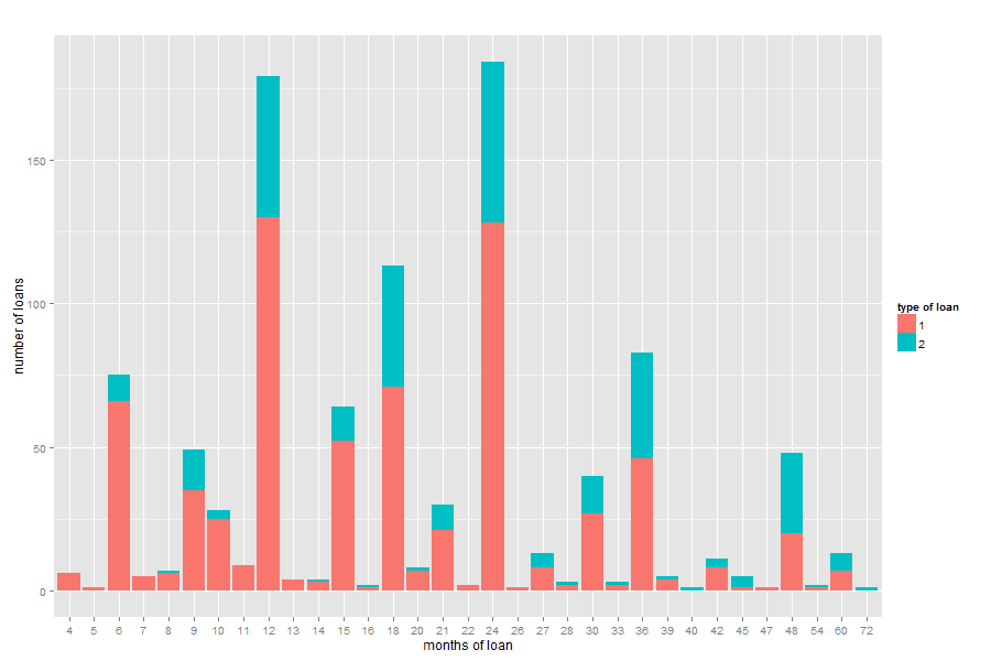
And suggests that the proportion of bad loans in relation to good loans tend to be larger for loans with durations greater than 36 months.
Now, let's take a look at the data preparation step. I would recommend to get rid of extreme outliers, null values, and missing values. It is not the case for this data set, as it seems to be purposely prepared for machine learning research.
For example, if it was the case, we could verify and eliminate missing values which are represented in R by the type 'NA':
for(i in 1:ncol(data)) print(which(is.na(data[,i])==T))
integer(0)
integer(0)
integer(0)
integer(0)
integer(0)
...
data <- na.omit(data)
Now let's see what is the proportion of good and bad credits:
round(prop.table(table(data$V25))*100, 2)
 1  2
70 30
This shows us that, from the 1,000 examples in the data set, 70% are examples of good credit and 30 % are examples of bad credit. We have to take that into consideration when we split this data set for training and testing our model. So, let's prepare our training set so that it contains the same amount of good and bad credit examples and see if its performance on the test set improves:
index <- sample(which(y_train==0),length(which(y_train==1)))
index <- c(index, which(y_train==1))
X_train <- X_train[index,]
y_train <- y_train[index]
Now let's check the proportion of good (0) and bad (1) credit on the train data to see if the splitting we want is correct. Notice that this step is performed after adjusting the outcome values for good and bad credit from 1 and 2 to 0 and 1 respectively, which is needed to perform binary classification with Logistic Regression:
round(prop.table(table(y_train))*100, 2)
y_train
 0  1
50 50
After running the training and test steps, we get the following results:
steps:  1351
corrects:  145
wrongs:  55
accuracy:  0.725
But let's see what really matters, the cross table results:
print(CrossTable(y_test,round(y_pred), dnn=c('y_test','y_pred'), prop.chisq = FALSE,
prop.c = FALSE, prop.r = FALSE))
...
Total Observations in Table:  200

             | y_pred
      y_test |         0 |         1 | Row Total |
-------------|-----------|-----------|-----------|
           0 |       104 |        39 |       143 |
             |     0.520 |     0.195 |           |
-------------|-----------|-----------|-----------|
           1 |        16 |        41 |        57 |
             |     0.080 |     0.205 |           |
-------------|-----------|-----------|-----------|
Column Total |       120 |        80 |       200 |
-------------|-----------|-----------|-----------|

$t
   y
x     0   1
  0 104  39
  1  16  41

$prop.row
   y
x           0         1
  0 0.7272727 0.2727273
  1 0.2807018 0.7192982
...
That is a lot of improvement in relation to the last results. By better balancing our training data we were able to reduce the misclassification of bad credits (classification of bad credit as good credit) from 75.4% to 28%. That was possible because the misclassification of good credits increased from 4.2% to 27.3%.
Now that our results are better balanced, let's see how our model performs with its own training data. With that, we aim to find out if the model is overfitting or underfitting the data:
y_pred <- hypot(X_train%*%theta)
print(CrossTable(y_train,round(y_pred), dnn=c('y_train','y_pred'), prop.chisq = FALSE,
prop.c = FALSE, prop.r = FALSE))
...
Total Observations in Table:  486

             | y_pred
     y_train |         0 |         1 | Row Total |
-------------|-----------|-----------|-----------|
           0 |       181 |        62 |       243 |
             |     0.372 |     0.128 |           |
-------------|-----------|-----------|-----------|
           1 |        63 |       180 |       243 |
             |     0.130 |     0.370 |           |
-------------|-----------|-----------|-----------|
Column Total |       244 |       242 |       486 |
-------------|-----------|-----------|-----------|

$t
   y
x     0   1
  0 181  62
  1  63 180

$prop.row
   y
x           0         1
  0 0.7448560 0.2551440
  1 0.2592593 0.7407407
...
It seems not be the case of overfitting, as the errors by scoring the training data are very similar when scoring the test data, for a relatively small number of examples to train on. We should investigating further to see if the model is underfitting, or if it is performing just rigth according to the given data.
Let's then analyze how the error in both the training and test data vary according to the number of examples in the training data, For that, we will plot the Mean Squared Error (MSE) of the predicted classes for both the training and test data, by the number of examples used for training the model. For that, we will vary our training data size from 25 to 550 examples, equally divided between good and bad credit classes. And we will separate 10% of the data set as the test data, keeping the original proportion of 70% of good credit and 30% of bad credit:

This learning curve seems not to be a typical curve of overfitting, as there is no gap between the train and test errors after a certain number of examples. Therefore, trying to address overfitting, by adding more examples or a Regularization factor in the cost function of Logistic Regression.
If it was a case of underfitting, we should try to come up with new relevant features that would help to better describe our data. This would be a task for someone with access to the right data and a good understanding of the credit business problem.
But even if we are not able to add more features, we can still have a better understanding of how the features we have at hand are able to describe our data. Two common approaches for that are Exploratory Factor Analysis for Feature Selection and Principal Component Analysis.
Trying to understand attribute importance through Exploratory Factor Analysis or Principal Component Analysis would allow us to identify the subset of variables that better describe our data and account for as much variability in the data as possible (in case such a subset exists).
Different from Feature Selection methods, Principal Component Analysis will create a new set of linearly uncorrelated features from the original set of variables, which is equal in size or less than the size of those original features.
It is out of the scope of this tutorial to dive deeper into the field of Exploratory Data Analysis. Nonetheless, I will show you some benefits that we can get when applying those techniques as a pre-processing step for our Logistic Regression classifier. The results bellow are averages of 50 independent runs of Logistic Regression:
=> using all original variables:
about 1300 steps to converge
error (good credit classified as bad):  0.2288
error (bad credit classified as good):  0.2421333
=> 12 most important original variables (from Feature Selection):
about 2400 steps to converge
error (good credit classified as bad):  0.184
error (bad credit classified as good):  0.2874667
=> 8 most important new features (from Principal Component Analysis):
about 250 steps to converge
error (good credit classified as bad):  0.1696
error (bad credit classified as good):  0.2888
We can clearly see that by applying Principal Component Analysis and choosing the 8 most important new derived features, we can further reduce the false positive error to 17%. This seems to be a very desirable effect to the credit business, even in the expense of increasing the false negative error a little bit.
Another desirable benefit of this approach is the simplification in the model. We are able to reduce the number of original variables from 24 to only 8 new features that seem to better model the data. With this simplification, the training process through Gradient Descent only takes 250 steps, instead of 1300 in the original setup.
©2014 - Alexandre Vilcek
Subscribe to:
Posts (Atom)